Basic course of thermo-fluid analysis

Chapter 1: Thermo-fluid analyses

This chapter describes basic phenomena about fluid flow and heat transfer. It also discusses some advantages and disadvantages of using CFD software.

1.1 Thermo-fluid-related phenomena

Air and water at room temperature are characterized by the fact that they flow without any specific shape. Substances with this characteristic are collectively called fluid .

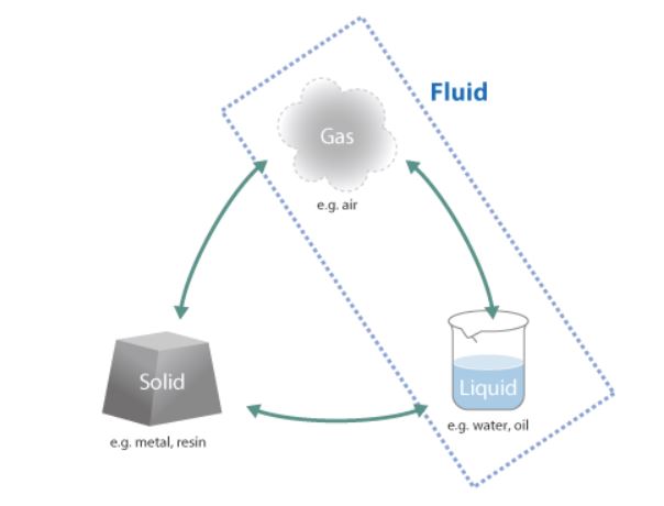
Figure 1.1: Three states of matter

A variety of fluids, such as air and water, exist on the earth. The flow of a fluid and heat transfer relate to many phenomena observed in our everyday lives.

• The air flow around automobiles and airplanes highly affects their performance.
• Electronic devices and electric circuits must be designed to readily release heat and keep the temperature below limit so the components won't overheat.
• Understanding the flow of air and heat in and around building structures is crucial for properly designing efficient air-conditioning systems to create a comfortable inside environment.

• The air flow around automobiles and airplanes highly affects their performance.
• Electronic devices and electric circuits must be designed to readily release heat and keep the temperature below limit so the components won't overheat.
• Understanding the flow of air and heat in and around building structures is crucial for properly designing efficient air-conditioning systems to create a comfortable inside environment. 
  
  

Figure 1.2: Phenomena related to the flow of a fluid and heat transfer

1.2 Advantages of CFD analyses

Prior to computational simulation, new designs were evaluated by running tests. Then, the test results and experience were used to dictate design modifications. The test results to drive design improvements use real world data, which is very reliable. However, running tests is expensive in terms of cost, time, and labor.

CFD software is a computational tool that helps overcome these obstacles. CFD stands for Computational Fluid Dynamics , which is the science of using the computer to simulate how fluids and energy flow. As analysis technology and computer performance improved, CFD accuracy improved. Today many companies routinely use CFD to design their products. Some of the advantages of CFD are as follows:

•  The effects of different operating conditions can be evaluated without creating prototypes. Development time and total cost can be reduced.
• Detailed data can be obtained even in places where experimental measurements may not be possible. Conditions can be simulated when it may be difficult or even nearly impossible to achieve data experimentally.
• The flows of a fluid and energy are difficult to visualize. However, CFD software provides a medium for seeing the invisible. Visualizing the computational results makes it possible to objectively explain phenomena.
• The following figures are some examples of CFD analyses.
  
  

Figure 1.3: Examples of CFD analyses

As you can see, CFD software has many attractive features. However, as with anything, it also has its weak points. For the simulation of a computationally intensive physical phenomenon, the physical model or object geometry may be simplified. Errors related to the simplification can occur. In addition, any numerical calculation by a computer always risks calculation error.

In conclusion, being fully aware of the advantages and disadvantages of using CFD software is crucial. In addition, the simulation results should be validated using measurement data to ensure the results are consistent with real-world phenomena and physics.

Chapter 2 Material Properties I

Chapter 2 Material Properties II

2.3 Specific heat

Specific heat is the amount of heat required to increase the temperature of a substance 1K for each unit mass of the substance. The unit of specific heat is J/(kg・K).

When the specific heat of an object is large, more energy must be applied to the object to increase its temperature. Likewise, more energy will be released from the object when it is cooled. An object with a large specific heat is hard to warm up and cool down.

Consider an iron frying pan and an earthen pot, that both weigh the same, on a stove. The iron frying pan warms up quickly while the earthen pot takes longer to warm up.

Figure 2.3: Difference of warming

In addition, when the stove is turned off, the iron frying pan cools down quickly while the earthen pot takes longer to cool.

Figure 2.4: Difference of cooling

The difference in the amount of time that it takes to heat and cool the iron frying pan and the earthen pot is caused by the difference in their specific heats. The specific heat of the earthen pot is about two times larger than that of the iron frying pan. Heat capacity indicates the amount of energy required to increase the temperature of an object 1K and is obtained by multiplying the mass of the object and the specific heat. The unit of heat capacity is J/K.

2.4 Thermal conductivity

When objects are at different temperatures, heat transfers from the hotter object to the cooler object. Thermal conductivity is the property of a material that determines how easily the heat moves within a material. The unit of thermal conductivity is W/(m・k). Consider a metal can containing a hot drink and a paper cup containing the same hot drink. The liquids are at the same temperature. When you hold each in your hand, the can feels hotter than the paper cup even though the drinks are at the same temperature. This is because the thermal conductivity of the metal can is higher than that of the paper cup. In other words, the metal can conducts more heat than the paper cup.

Figure 2.5: Difference of heat conduction

Chapter 3 Basics of Flow I

Chapter 3 discusses parameters used to describe flows. The units used in this chapter conform to the SI unit system.

3.1 Describing flows

A flow is the movement of a fluid. Fluids can be either liquids or gases. For gases, the gas flow is often invisible. Therefore, flows must be described in some form. This chapter introduces the typical parameters used to describe flows. These parameters will help you visualize the movement and behavior of the invisible flows.

3.1.1 Velocity, speed, and flow rate

Velocity and speed describe the rate of the movement of a fluid per unit time, and the unit is m/s. When the term fluid velocity is used, it indicates both magnitude and direction of movement. Velocity is called a vector quantity because it contains these two pieces of information. On the other hand, speed only specifies “the magnitude of fluid velocity”. Speed is a scalar quantity, It specifies the magnitude and has no directional information.

Figure 3.1: Magnitude and direction of velocity

Flow rate is the volume of a fluid passing through a cross-section per unit time. The unit of flow rate is m3/s. Flow rate is also called volumetric flow rate, and is obtained by multiplying the area of the cross-section through which the fluid passes by the velocity of a flow normal to the cross-section. If we multiply the volumetric flow rate by the density of the fluid passing through a cross-section per unit time, this is called the mass flow rate. Its unit is kg/s.

Figure 3.2: Velocity and flow rate

3.1.2 Pressure

Pressure is the amount of force acting on a unit surface area, and its unit is Pa. The force (unit: N) is obtained by multiplying the pressure by the area on which the pressure acts. The standard atmospheric pressure on the ground is 101,325 Pa. This is equivalent to a 10 metric tons (t) object on an area of 1 m2.

Figure 3.3: Standard atmospheric pressure

Chapter 3 Basics of Flow II

3.1.3 Streamlines, streaklines, and pathlines

Visualizing flow using streamlines, streaklines, or pathlines makes it more intuitively understandable.

A streamline is a line which smoothly connects velocity vectors at an instance in time. In other words, an image of the flow characterized by streamlines is like a snapshot of the flow at one moment in time.

Figure 3.4: Streamline

A streakline is a curved line formed by a string of fluid particles which have passed through a certain point. An example of a streakline is the trail of smoke from a chimney.

Figure 3.5: Streakline

A pathline is a path which a fluid particle traces. One example of a pathline is the path defined by a balloon floating in the air.

Figure 3.6: Pathline

For a flow which does not change with time, the streamline, streakline, and pathline are the same line. A flow which does not change with time is called a steady-state flow . On the other hand, a flow which varies with time is called a transient flow. For transient flows, the streamline, streakline, and pathline are all different lines.

Figure 3.7: Example of streamlines

A streakline represents all the points that have passed through a certain location. For this situation, where the streakline can be likened to represent the smoke trail from a chimney, the streakline goes to the south during the first 10 seconds because all the smoke is going south. Then, when the wind shifts to the east, all the smoke particles that were initially heading south (emitted for Time < 10 seconds) start to be offset to the east. The newer smoke particles (emitted for Time > 10 seconds) head directly east. After 20 seconds the streakline is at a right angle as shown on the right in Figure 3.8.

Figure 3.8: Example of a streakline

A pathline goes to the south during the first 10 seconds just as the streakline. The pathline can be thought of as the path traced by a balloon floating in the air. When the wind shifts to the east, the balloon starts moving east. The pathline goes to the east from the point where the wind direction has been changed. As a result, after 20 seconds the pathline bends at a right angle as shown on the right in Figure 3.9.

Figure 3.9: Example of a pathline

As can be seen in this chapter, the analysis results for transient flows will be different depending on the method used to visualize the flow. Understanding this difference is important when visualizing analysis and experimental results.

Chapter 3 Basics of Flow III 

3.2 Characteristics of flows

This chapter introduces some of the important characteristics of a flow. The difference in flow characteristics may affect how the flow is analyzed. In addition, knowing the flow characteristics is very important when evaluating the validity of an obtained result.

3.2.1 Compressible/incompressible fluids

Compression and expansion are important characteristics of a fluid. Remember that a fluid can be a liquid or a gas. If compression and expansion have a significant effect on the fluid density (kg/m3), the fluid is called a compressible fluid. Consider a simple example of a gas in a cylinder as shown in Figure 3.10. The cylinder is sealed so that gas cannot enter or escape. The fluid volume changes as the piston moves. However, the mass of the system does not change because the gas is not allowed to enter or leave the cylinder. Therefore, the fluid density must change because of the change in volume.

Figure 3.10: Compressible fluid

On the other hand, when compression and expansion do not significantly affect the fluid density, the fluid is called an incompressible fluid. The volume of an incompressible fluid does not change and its density is treated as a constant. Consider a liquid in a cylinder. If the cylinder is sealed, the piston will stop moving once it contacts the liquid. As the piston retracts, an empty space is created above the liquid surface. The amount of space (volume) the liquid occupies does not change (actually the volume does change but the change is very tiny). Since the amount of the liquid is almost unchanged, the fluid density (kg/m3) is constant. Liquids are always considered to be incompressible fluids, as density changes caused by pressure and temperature are small.

While intuitively gases may always seem to be incompressible fluids if the gas is permitted to move, a gas can be treated as being incompressible if its change in density is small. Consider the cylinder filled with a gas as shown in Figure 3.11. Ports are added to the cylinder that permits gas to enter or leave the cylinder. As the piston pushes down, the gas flows out of the port because the volume of the cylinder decreases. The amount of mass of the gas also decreases proportionally, and the density of the gas (kg/m3) in the cylinder is unchanged. When the piston retracts, the volume of the system increases, gas (mass) enters through the port and the density of the gas (kg/m3) remains again essentially constant. In this situation, the gas behaves as an incompressible fluid. In a strict sense, a completely incompressible fluid does not exist. However, when the density changes due to pressure (the movement of the piston applies pressure to the fluid in the cylinder) or temperature is small, approximating a fluid as an incompressible fluid can greatly simplify calculations.

Figure 3.11: Incompressible fluid

One measure of the degree of compressibility of a gas is the Mach number M of the flow. The Mach number is the ratio of the fluid velocity to the speed of sound. When M < approx. 0.3, a fluid can be treated as incompressible. For an air temperature of 20°C, the speed of sound is approximately 340 m/s. Therefore, if the fluid velocity is 100 m/s or greater, compressibility should be considered in the calculations. For fluid velocities less than 100 m/s, the fluid can be considered incompressible. In addition, if the fluid temperature changes significantly (this is different than the fluid being at a constant high or low temperature), the fluid density will also change substantially during volume expansion or compression. In this case, the fluid may also be treated as a compressible fluid.

Chapter 3 Basics of Flow IV

3.2.2 Steady state and transient state

Consider the situation where water is poured into a container which has an outlet part on the side of the container as shown in Figure 3.12. At first when the water level is below the outlet, the water level in the container rises with time as shown in (a). However, when the water level reaches a certain height, the amount of water entering the tank and the amount of discharged water are balanced and the water level remains constant (See [b]).

Figure 3.12: Water level change

When the state of the system changes with time, this is called the transient state as shown in [a]. On the other hand, when the state is constant with time, this is called the steady state. You must identify the correct state before performing a thermo-fluid analysis.

In a steady-state analysis, only a steady-state solution is obtained. The analysis cannot predict how the process achieved the steady-state condition. If the thermo-fluid analysis is terminated before the analysis reaches the steady-state solution, the result does not have any physical meaning.

On the other hand, a transient analysis accurately calculates the system conditions as it changes with time. Therefore, the transient analysis calculates the time variation of a phenomenon. If the transient analysis is permitted to run for a long enough time, the steady-state solution will eventually be obtained. The steady-state solution will generally be obtained by using a steady-state analysis much faster than transient analysis. Therefore, if the steady-state solution is all that is needed, the calculations should be performed as a steady-state analysis.

3.2.3 Bernoulli's theory

When the fluid density is designated by the Greek symbol ρ (rho) and fluid velocity by the letter ν, the unit for ρν2/2 is the same as that for pressure. This expression represents the kinetic energy of a fluid flow and is called the dynamic pressure. In contrast, a force such as atmospheric pressure that acts on the system is called static pressure. The sum of the dynamic and static pressures is called the total pressure.

Imagine a fluid does not have any viscosity and its volume does not change. This fluid is called an ideal fluid. When the flow of an ideal fluid does not change with time, its total pressure is constant. This is called Bernoulli's theory and expresses the fluid energy conservation law. In a real flow, energy is lost due to viscosity and the total pressure decreases in the flow direction.

Consider the flow at cross-sections A and B in Figure 3.13. For an ideal fluid, the total pressure at the two cross-sections is the same as explained by Bernoulli’s theory. At cross-section A, where the area is larger, the flow velocity is lower compared to the flow velocity at cross-section B. The total mass flow is constant. Therefore, the dynamic pressure at cross-section A < dynamic pressure at cross-section B. In turn, the static pressure at cross-section A > static pressure at cross-section B since the total pressure is constant.

Figure 3.13: Bernoulli’s theory

A simple experiment can illustrate the Bernoulli theory. Consider two balloons as shown in Figure 3.14. Strongly blow in the space between the balloons. The balloons will come together and may even contact each other. According to Bernoulli’s theory, the balloons come together because the static pressure decreases when the velocity increases.

Figure 3.14: Experiment using balloons

Chapter 3 Basics of Flow V

3.2.4 Laminar flow and turbulent flow

A flow has two states: laminar and turbulent. A fluid flow with regular, predictable motion is called laminar flow. On the other hand, a flow with irregular, unpredictable motion is called turbulent flow.

Consider water running from a tap to illustrate the two states. When the tap is turned on just a small amount, water flows straight down in a very well-behaved and predictable stream as shown in (a) of Figure 3.15. The more the flow increases the more turbulent the water flow becomes. The surface of the water creates waves as shown in (b).

Figure 3.15: Water running from a tap

In 1883, a British scientist named Osborne Reynolds (1842-1912) classified flows as either laminar or turbulent from a series of experiments known as the Reynolds’ experiment. In the experiment, flows were visualized by pouring a stream of ink into a pipe in which water flows. The result showed that, when the water velocity was low, the ink moved downstream in a continuous straight line as shown in (a) of Figure 3.16. In this case, the flow was laminar. However, when the water velocity was high, the ink started in a straight line but began oscillating and quickly dispersed throughout the pipe. This flow was turbulent.

Figure 3.16: Reynolds’ experiment

In the experiment, Reynolds discovered a dimensionless number could be used to classify flows as either laminar or turbulent. This number is called the Reynolds number. The Reynolds number Re is defined by the following equation:

where,

L: Characteristic length
       (In this example, L is the inside diameter of the pipe)
U: Representative velocity
       (Here, it is the average velocity of the flow passing through a cross-section of the pipe)
ρ : Fluid density
μ: Viscosity coefficient

The denominator of the equation expresses the viscous force of the fluid. The numerator of the equation expresses the inertial force. Hence, the Reynolds number is the ratio of the inertial force to the viscous force. When two flows are geometrically similar and have the same Reynolds number, this means their ratio between their inertial forces and their viscous forces will be the same. Thus, the behavior of the two flows will be essentially the same. This law is called the Reynolds' law of similarity.

Consider another example. Suppose you want to simulate the air flow around an automobile moving at a speed of 50 km/h by using a half-size model in a wind tunnel as shown in Figure 3.17. The equation for the Reynolds number says the air velocity should be 100 km/h since the characteristic length has been cut in half to maintain a constant Reynolds number.

Figure 3.17: Reynolds' law of similarity

A closer look at the Reynolds number reveals the following: When the fluid viscosity is large or the fluid velocity is low, the viscous force becomes dominant. When this occurs, the Reynolds number will be small and the fluid flow will be laminar. On the other hand, when the fluid viscosity is small or the velocity is high, the inertial force becomes dominant. Thus, the Reynolds number of the fluid will be large and the fluid flow will be turbulent.

The range of Reynolds number for the transition from laminar to turbulent flow in a pipe is generally 2,000 to 4,000. These values are just approximated and the actual values will vary depending on the state or conditions of the flow.

In this final example, we can determine whether the air flow around a bicyclist is laminar or turbulent. Figure 3.18 shows the air flow around a bicyclist traveling at 14.4 km/h.

Figure 3.18: Person riding on a bicycle

The Reynolds number is calculated using the following equation for the flow of air.

The calculated value for the Reynolds number is 400,000, far greater than the aforementioned approximate value of 2,000 - 4,000 denoting the conditions when the flow transitions from laminar to turbulent. We find that the majority of flows observed in our daily lives is turbulent.

A turbulent flow can be either an advantage or disadvantage. A turbulent flow increases the amount of air resistance and noise; however, a turbulent flow also accelerates heat conduction and thermal mixing. Therefore, understanding, handling, and controlling turbulent flows can be crucial for successful product design.

Chapter 4 Basics of Heat I

This chapter describes four aspects of heat: temperature and heat, buoyancy, natural and forced convections, and heat transfer. All units are SI units.

4.1 Temperature and heat

Temperature is the numerical measure of hot and cold. Its units are [°C] or [K]. Celsius temperature uses the unit [°C] while absolute temperature uses [K]. One degree in both temperature scales represents the same temperature difference. However, the base temperatures for the two scales are different. The relationship between the two temperature scales is expressed by the following equation:

A temperature of 0 °C is equal to 273.15 K.

An object can possess internal energy which is represented by its temperature. Heat is one form of the internal energy. When heat flows into an object, its temperature rises. When heat flows out of an object, its temperature decreases. The amount of heat is expressed in joules [J]. The amount of heat per unit time is expressed in watts [W]. Consider a room in the winter. As shown in Figure 4.1, when the heater is turned on, the room temperature rises. The heat from the heater is transferred to the air in the room, and the room air temperature rises.

Figure 4.1: Heat transfer when the heater is on

Figure 4.2 shows when the heater is turned off, the room temperature decreases. This is because heat is transferred from the air inside the room to the outside air causing the room air temperature to decrease.

Figure 4.1: Heat transfer when the heater is off

Heat transfers from objects with a higher temperature to objects with a lower temperature. When two objects with different temperatures are in contact with each other, their temperatures eventually become equal.

4.2 Buoyancy

When the temperature of a fluid increases, the molecules (atoms) within the fluid move around more actively. As a result, the volume of the fluid increases and the density of the fluid decreases. When a fluid is heated, a force opposite of gravity occurs due to the density difference. This force is called buoyancy. A hot-air balloon, as shown in Figure 4.3, is a typical example of buoyancy.

Figure 4.3: Principle of hot-air balloon

Buoyancy of a compressible fluid can be treated in a straightforward manner because the volume is inversely proportional to the temperature. On the other hand, the volume change of an incompressible fluid is difficult to quantify. Because of this, the buoyancy of an incompressible fluid is approximated using a force that is proportional to temperature difference. This approximation is called the Boussinesq approximation. The error caused by the Boussinesq approximation is large when the temperature difference is very large.

4.3 Natural convection and forced convection

The flow of fluid is classified in two ways depending on what is driving the flow. The two methods are: natural convection and forced convection.

With natural convection, heat flows without any assistance from external sources, e.g. a fan or pump. Natural convection is driven by buoyancy which is caused by differences in the fluid temperature. On the other hand, with forced convection, heat flow is caused by an external source such as a fan or pump, which moves the fluid. In (a) of Figure 4.4, a container of water is heated, and the heated water starts rising from the bottom of the container to the top of the container due to buoyancy. This is natural convection. On the other hand, as shown in (b) of Figure 4.4, when the water in the container is stirred with a stick, a flow is created which is caused by an external factor. This is an example of forced convection.

Figure 4.4: Natural convection and forced convection

For forced convection, the buoyancy effect is small compared to the inertia force. This is a characteristic of flows driven by an external force such as a fan. Because the buoyancy effect is so small, it does not need to be considered in some analysis cases. However, in a flow with only natural convection or a flow with equal natural and forced convections, buoyancy effect cannot be ignored.

Chapter 4 Basics of Heat II

4.4 Forms of heat transfer

There are three forms of heat transfer: conduction, convection, and radiation. Consider a room as shown in Figure 4.5. You will feel warmth where you contact the heated floor because of conduction. You will feel warm wind from the heating unit due to convection. You will feel warmth in front of the stove due to radiation. Each form of heat transfer will be explained in more detail below.

Figure 4.5: Form of heat transfer

4.4.1 Conduction

When the temperature in an object is uneven, the atoms and molecules (including the free electrons in metals) move within the object. Heat is transferred from the higher temperature region to the lower temperature region. This type of heat transfer is called thermal conduction.

For example, as shown in Figure 4.6, when you hold a can of hot tea, you feel the heat through the can. This is because heat is thermally conducted through the can due to the temperature difference between the hot tea and your cooler hand.

Figure 4.6 Heat transfer by conduction

Thermal conductivity is the property of a material that determines how much heat is transferred within an object. For two materials with the same initial temperature difference across them, the material with the higher thermal conductivity will reach a uniform temperature more quickly.

Heat conduction is a phenomenon that enables heat to be transferred within an object. Heat conduction can occur in solids, not only in fluids such as liquids, and gases.

4.4.2 Convection

In heat conduction, heat is transferred within an object. When the object is a fluid, heat can be transferred from the fluid to another object by flow of the fluid on the surface of the object. This type of heat transfer is called convection. Convection can transfer larger amounts of heat than conduction.

For example, as shown in Figure 4.7, when a container with water in it is heated, conduction heat transfer occurs within the water at the bottom of the container. In addition, the heated water rises due to buoyancy and convection occurs along the sides of the container, which leads to additional heat transfer.

Figure 4.7: Heat transfer by convection

The heat transfer coefficient expresses the amount of heat transferred between a fluid (either a liquid or gas) and a solid surface by convection. Heat can move from the fluid to the surface or vice versa. The heat transfer coefficient depends on a kind of fluid, its flow state, and the shape of the object. The larger the heat transfer coefficient, the more heat transfer occurs.

In general, the larger the thermal conductivity for a fluid, the larger the heat transfer coefficient. Therefore, the heat transfer coefficient for a liquid is higher than that of a gas.

For example, you can enjoy a sauna with an air temperature of 100 °C, but you cannot enjoy a bath with a water temperature of 100 °C. This is because the heat transfer coefficient of water is higher than that of air. The liquid water will transfer more heat to your skin than the air in the sauna. As a result, you will feel much hotter in the water than in the air.

Another factor that greatly influences the magnitude of the heat transfer coefficient is the fluid flow velocity over the object surface. The higher the velocity, the larger the heat transfer coefficient. Therefore, the heat transfer due to forced convection is larger than that of natural convection. The strong breeze from an electric fan will cool you faster than when no fan is present.

Chapter 4 Basics of Heat III

4.4.3 Radiation

When the atoms and molecules within an object move, some of their internal energy is released in the form of electromagnetic waves. In contrast, when an object receives electromagnetic waves, it absorbs the energy and converts it into internal energy. Heat transfer via electromagnetic waves is called radiation heat transfer.
For both conduction and convection, a medium is needed to transfer energy. Conduction transfer energy through a material. Convection transfers energy though a fluid. In contrast, radiation does not require a medium to transfer energy. Radiation heat transfer can occur in a vacuum such as outer space.
Consider Figure 4.8 where the temperature on the roof and the street is higher than the air temperature on a sunny day. This is because electromagnetic waves released from the sun directly warm up the surfaces of the roof and the street, and pass through outer space and air.

Figure 4.8: Heat transfer by radiation

Emissivity is a characteristic of a solid, liquid, or gas, and expresses the rate that the material absorbs or releases energy by radiation. The range of emissivity is 0 ~ 1. The greater the value, the more energy is absorbed or released due to radiation. If a material has an emissivity of 1.0, this means the material will absorb all the radiation energy that hits its surface. None of the energy will be reflected from its surface. In addition, if a heated material has an emissivity of 1.0, this means the material will radiate the maximum amount of energy from its surface. Emissivity varies depending on the material and/or a color on the surface of an object. In general, emissivity is high for a black object and low for a white object or a well-polished (reflective) surface.

View factor is another important parameter in radiation heat transfer. It expresses the proportion of total energy which is released from one surface and reaches the other surface. The view factor is determined from the geometric shape of two heat transfer surfaces. The value of the view factor ranges from 0 ~ 1. If the receiving surface is completely visible, the view factor is 1. If it is not visible, the view factor is 0.
In Figure 4.9, Surface 2 can be seen from Surface 1 in all direction (blue lines). Therefore, the view factor from Surface 1 to Surface 2 is 1. On the other hand, only part of Surface 1 can be seen from Surface 2 (red solid lines). Part of Surface 1 cannot be seen from Surface 2 (red dashed lines). Therefore, the view factor from Surface 2 to Surface 1 is less than 1. An important point to note is that the view factor between two surfaces will often not be the same value.

Figure 4.9 Example of view factor

The higher the emissivity of two surfaces at different temperatures and the larger the view factor, the larger the amount of heat transfer by radiation between the surfaces.

Chapter 5 Basics of thermo-fluid analyses I

This chapter describes basic concepts and procedures for thermo-fluid analyses.

5.1 Fundamental equations and discretization

Transfer or motion of a fluid or heat is expressed by differential equations. For incompressible fluids, which are mainly considered here, the following equations are fundamental:

• Navier-Stokes equations (Momentum equations)
• Equation of continuity
• Energy conservation equation

The Navier-Stokes equations and the continuity equation express the motion of a fluid, while the energy conservation equation expresses the motion of heat. These equations are fundamental for thermo-fluid analyses, and are called governing equations (or fundamental equations ).

If the fundamental equations can be analytically solved, the distributions of heat, temperature, and flow can be explicitly obtained. However, the equations are sufficiently complex and analytic results have only been obtained for very limited cases. As an alternative, thermo-fluid analysis uses the computer to numerically solve the fundamental equations. However, a computer can only process discrete values and cannot process continuous values as is illustrated in the following example.

To understand the aforementioned topic more easily, let us think about a calculator.

A calculator can obtain the results of an equation “y = x + 1”, for example, by calculating as follows:

If x = 1, y = 1 + 1 = 2
If x = 2, y = 2 + 1 = 3
If x = 3, y = 3 + 1 = 4
:
:

As shown above, a calculator can obtain a calculation result for discrete input values.

However, it cannot process a function, which is a series of continuous or infinitely small values.

To solve this problem, the fundamental equations must be transformed into expressions composed of discrete values. This transformation is called discretization.

Figure 5.1: Example of discretization

To help understand discretization intuitively, consider the weather. The weather varies continuously in space, so it cannot be easily processed, as is, by computer.

Figure 5.2: Actual weather in three cities

To process the weather using a computer, first determine a specific location where the weather will be characterized. Then, develop relationships that characterize the change in the weather between the specific location identified and the surrounding area. This process corresponds to discretization. Assume the obtained relation is as follows: The weather at any point is given by averaging the weather at surrounding points. According to this relationship, when the weather in Yokohama and Omiya are sunny and rainy, respectively, the computer calculates their average and determines the weather will be “cloudy” in Tokyo.

Figure 5.3: Weather processed by computer

A simple average is used in the aforementioned example; however, more complicated relationships are used to describe thermo-fluid relationships between a specific point in space and the surrounding points in a thermo-fluid analysis. There are a few different discretization methods but the major ones are:

• Finite Difference Method (FDM)
• Finite Volume Method (FVM)
• Finite Element Method (FEM)

Many commercial thermo-fluid software products use the finite volume method for discretization. (The finite volume method is explained in the next chapter.) So while the fundamental thermo-fluid equations are differential equations (which by definition correspond to an infinitesimally small difference between neighboring “points”), discretization enables expressing the relationships between neighboring spaces with algebraic equations (equations that can be expressed using basic arithmetic operations).

To simulate thermo-fluid phenomena such as the flow of the wind around buildings, air flow over a car or the temperature distribution in a room in a thermo-fluid analysis, the target space must be first divided into tiny regions called elements or cells. Then, the fundamental equations for thermo-fluid flow which have been discretized using one of the methods listed above, along with assigning appropriate boundary and initial conditions can be solved numerically. The result is solution of the flow velocity and pressure distributions from the Navier-Stokes and continuity equations, and the temperature from the energy conservation equation.

5.2 Finite volume method

The finite volume method (FVM) is a method for estimating the amount of a physical quantity stored in a space based on the difference between the amount of inflow and outflow to the space.

Consider the situation where water is poured into a container as shown in Figure 5.4. The amount of water (variation) that accumulates in the container over a certain period is obtained from the difference between the amount of inflow and outflow. When the amount of accumulated water is determined, the change in the water level can be calculated knowing the dimensions of the container. This change in water level is an example of how a physical quantity is calculated using the finite volume method.

Figure 5.4: Concept of finite volume method

In an actual analysis, the analysis target is divided into many small containers or spaces. The containers are connected as shown in Figure 5.5.

Figure 5.5: Analysis target is divided into multiple spaces

The amount of outflow from one container is equal to the amount of water flowing into the next container.

Now, let's take a more concrete example. To obtain the temperature from the energy conservation equation, consider the amount of heat flowing into a space due to thermal conduction and heat convection, and the amount of heat flowing out from the space. The goal is to obtain the temperature variation (change in temperature) from the amount of stored heat.

Figure 5.6: Inflow and outflow of heat

The inflow and outflow of heat are calculated for each space and the amount of stored heat for each space is calculated from these values. Once the amount of stored heat is known for each space, temperature in each space can be calculated.

Figure 5.7 is used to conceptually illustrate the calculation process for achieving the steady state temperature of a part that is heated at one end. The left end is at a high temperature and the right end is at a low temperature. Initially the temperatures between the two ends are unknown. Starting from the left end, the temperature gradually rises in the adjacent spaces as heat flows from a space of higher temperature to that of lower temperature. The amount of heat flowing into each space is greater than the amount of heat flowing out just after the start because the temperature difference between the first two cells on the left is higher than the difference between any of the other adjacent cells. After a sufficiently long time has passed, the amount of heat flowing into and out from each space is balanced as shown in the bottom of the figure* . Here, the temperature does not change and the steady state condition is achieved.

* The state corresponds to the state where the amounts of inflow and outflow in all the containers are balanced (water level does not change) in Figure 5.5.

Figure 5.7: Heat transfer and temperature distribution

This basic concept also applies to flows. The velocity change in each space is obtained by considering both the momenta flowing in and out of the space but also viscosity and pressure effects.

Figure 5.8: Inflow and outflow of momentum

Note that there is no governing equation to solve for pressure. To obtain pressure, other methods are used. For example, the fluid velocity can be calculated using an estimate of the pressure. Then the pressure is corrected such that the obtained velocity satisfies the equation of continuity.

5.3 Computational domain

Let's think about analyzing the air flow around an airplane in flight. To analyze the real flow perfectly, unlimited space would be needed because the space around the airplane consists of the sky and then outer space. Unfortunately, the computer must process a finite number of values.
Therefore, an appropriate and finite analysis space or area must be defined around the airplane and this space is called the analysis domain.

Figure 5.9: Computational domain

The faces of the computational domain are not solid walls, and they are created just to define a physical boundary for the calculation. Therefore, the computational domain must be large enough so that its faces are sufficiently far from the target object to prevent the faces of the computational domain from artificially influencing the flow over the object. For example, when some of the flow is outside the computational domain and flows back into the computational domain as shown in the lower right part of Figure 5.10 (a Bad example of defining the boundaries of the domain), the flows shown by the dotted lines are not correctly simulated. Consequently, the calculated result will likely be different from the real result. On the other hand, while it may seem simpler to select a very large domain, specifying an unnecessarily large domain will require much more time to obtain the solution.

Figure 5.10: Creating a computational domain

Determining the appropriate size of a computational domain can be challenging but becomes easier as the analyst gains more experience and an increased understanding of how flows behave.

5.4 Division of a space

The relationship between flow variables in neighboring spaces is calculated by discretizing the equations (e.g. momentum, energy, and continuity equations). Discretizing requires dividing the computational domain into many tiny spaces where each space is called an element or cell . The equations are expressed as functions of the geometrical relationships between adjacent cells. A set of elements or cells is called a mesh or grid .
Parameters, such as fluid velocity and temperature , are calculated for each element, and each element has one value for each parameter. The value of the parameter is constant within the entire element. Hence, resolution is improved as the elements become smaller. Figure 5.11 is an example of an analysis result where the temperature is high at the center of the model and low at its periphery. The figure shows that the larger the elements are, the larger the range can be for the parameter in the element (maximum – minimum value within the element). In other words, the parameter distribution will be coarser as the element size increases.

Figure 5.11: Element size and the analysis result

In general, the calculation requires less time for larger elements (fewer total elements) because fewer calculations must be performed. However, the calculation result will be less accurate due to the coarser distribution of the parameters. In contrast, the calculation will require more time for smaller elements (more total elements because more calculations must be performed. However, the calculation result will be more accurate and provide better resolution.

In many cases, a finer mesh is generated around the selected features in the model where the flow and temperature vary rapidly (large gradients). On the other hand, a coarser mesh can be used where flow and temperature vary slowly.
There are two meshing methods as shown in Figure 5.12. Elements are placed in a repeatable pattern in a structured mesh (left) and irregularly in an x /dcms_media/image/en_column_basic_unstructured mesh   (right).

Figure 5.12: Mesh generation

Figure 5.13 shows the element types most generally used in each meshing method.

Figure 5.13: Typical element types

In a 3D analysis, the structured mesh elements are hexahedrons, and they are placed in a repeatable pattern. This mesh is easily generated and the calculation speed is very fast. On the other hand, an unstructured mesh uses tetrahedrons and pentahedrons shaped elements. Mesh generation is more challenging compared to a structured mesh; however, the elements can be placed much more freely. Therefore, unstructured mesh is suitable for representing complicated geometries.

5.5 Boundary conditions

The value of a parameter within an element is calculated from the values for that parameter in the neighboring elements. For example, in Figure 5.14, the values for the elements shown in blue are used to calculate the value for the element shown in red.

Figure 5.14: Element surrounded by other elements

However, when an element is at the edge of the analysis domain as shown by the red element in Figure 5.15, the value for the element cannot use this method because one of the neighboring elements is missing. In this case, a value must be assigned for each parameter along the edge of the computational domain which corresponds to the edge of the element. The values assigned along the edges of the computational domain are called boundary conditions.

Figure 5.15: Element at the edge of the computational domain

In thermo-fluid analyses, fluid velocity, pressure, and temperature are typical boundary conditions. For example, if the wind is blowing into the computational domain, the values for the wind velocity and inflow temperature are the boundary conditions for the model.
There are three major types of boundary conditions:

• Dirichlet boundary condition

The Dirichlet boundary condition specifies the values of a boundary directly. Conditions such as “Velocity: 5 m/s”, “Pressure: 0 Pa”, and “Temperature: 20°C” are considered Dirichlet boundary conditions

Figure 5.16: Dirichlet boundary condition for a flow

• Neumann boundary condition

The Neumann boundary condition is a condition that specifies the gradient of the parameters. The gradient can be thought of as the rate of change. Conditions such as a free-slip condition and an adiabatic condition are examples of Neumann boundary conditions.
For example, consider an adiabatic condition as shown in (a) of Figure 5.17. When the temperatures at two points are different, heat transfers from the point with higher temperature to the point with the lower temperature. An adiabatic condition means no heat is transferred. This is achieved by having the temperatures of the two points be the same (see [b] of Figure 5.17). When the temperatures of the two points are the same, the temperature gradient (rate of change) is 0. Therefore, an adiabatic condition can be expressed by a Neumann boundary condition with a temperature gradient equal to 0.

Figure 5.17: Idea of adiabatic condition

• Periodic boundary condition

A periodic boundary condition sets the same values for a parameter on two or more faces. It is used to simulate periodicity (repetition) of the distribution. For the fan shown in Figure 5.18, the fan has four blades equally spaced around the center hub. The flow around each blade should be almost the same for all the blades. A periodic boundary condition can be applied to the boundary faces of one of the blades. This is used to simulate the motion of the entire fan by only modeling one blade. Note that there are certain times when the periodic boundary condition cannot be used. For example, a very high speed flow may not be periodic even though the geometrical model appears periodic.

Figure 5.18: Example of a periodic boundary condition

To perform an analysis properly, selecting the appropriate boundary condition is critical. If an improper boundary condition is assigned, the physical phenomena will not be properly simulated, resulting in erroneous results. Moreover, the calculation may also be unstable.

5.6 Initial condition

The condition that defines the initial state of an analysis is called an initial condition. For example, if the ambient temperature at the start of an analysis is 25°C, this is its initial state. “Temperature: 25°C” is set as an initial condition.

The initial condition is important particularly for a transient analysis. Figure 5.19 shows an environment at 20° C with two objects, whose temperatures are 50° C and 100° C, respectively placed in the environment. The object temperatures at the initial state are different. The temperatures are also different after five minutes as shown in the figure. Different initial conditions will make the calculation progress differently in a transient analysis.

Figure 5.19: Initial temperature and time variation of temperature

However, in both cases shown in Figure 5.19, the object temperature will be 20°C after a sufficient time. This is the same temperature as that of the surrounding space. This is the temperature that would be achieved for a steady-state analysis. The initial condition does not affect the calculation results for a steady-state analysis.
The same can be said of other variables besides temperature. If the calculated results are different for two steady-state analyses with different initial conditions, either or both of the calculations may not have reached steady state yet.

Note that the calculation time will be reduced for a steady-state analysis by setting the initial conditions, for each cell where parameter values are calculated, close to the anticipated steady state solution values.

5.7 Matrix solver

As seen in the previous section, the parameter values of each element are determined as a function of the values in the neighboring elements. For example, consider Element3 shown in Figure 5.20. The following expression is satisfied.

Figure 5.20: Positional relationship of an element with neighboring elements, and the relationship equation

This is a two-dimensional example. Element3 contacts with four total elements on the left, right, top, and bottom. For a three-dimensional example, the neighboring elements of Element3 would be not only the aforementioned four elements but also two more elements at the front and back of Element3. Therefore, for the three-dimensional example, the total number of the neighboring elements is six. For the flow equation, the constant is the external force acting on Element3 while the rate of heating is the constant for the thermal equation.

This relationship equation is created for each element. Therefore, if the model consists of one million elements, one million simultaneous linear equations with one million unknowns per variable would have to be solved. The group of equations can be expressed in matrix form and the solver used to determine the solutions to the equations is called the matrix solver. One of two different solver methods is commonly used. The first method is called the direct method, and the second method is called the iterative method. In a thermo-fluid analysis, the iterative method is generally used. Consider this example. A simultaneous system of linear equations with two unknowns is solved using the Jacobi iterative method.

The exact solution to this system of equations is x = 3 and y = 4. For a better understanding of how the solution is obtained iteratively, the system (1) is transformed as shown below:

To solve the system (2) by using the iterative method, give x and y initial values. Here, zero is entered initial values for x and y.

For the first iteration, the solution is x = 1 and y = 1. When this solution is substituted back into system (2) :

The second iterated solution is x = 1.5 and Y = 2. The process is repeated as shown in Figure 5.1 until the change in the solution values becomes very small, closer to the exact solution.

Figure 5.1: Calculation results using Jacobi method

In this example, the Jacobi method was used because of its simplicity. However, for practical problems with millions of elements and requiring hundreds of iterations, higher-speed iterative methods are needed.

As the number of iterations increases, the calculated result gets closer to the exact solution. However, for real world problems, obtaining the exact solution by iterating is difficult to achieve. Therefore, for most problems, the calculations are terminated when the difference between the calculated results for k-1th and kth calculations is less than a predetermined value. Then, the kth calculation result is used as the solution. The predetermined value is called the convergence criterion. Be aware that if the calculation does not converge sufficiently, i.e. the difference between the k-1thand kth calculations does not approach the convergence criterion, the correct solution may not be obtained.

5.8 Progress of time

There are two types of analyses: a steady-state analysis and a transient analysis.

In a steady-state analysis, only the final state is obtained without any change over time. In fact, time does not have any meaning in a steady-state analysis. Because of this, the states before the calculation reaches the final state do not have any physical significance. This is all another way of saying that only the final state has meaning in a steady-state analysis.

On the other hand, in a transient analysis, the analysis is separated by short time intervals. The state of a phenomenon from one moment to the next is calculated and the procedure is repeated. The states for each calculation step are determined, and represent the physical conditions at that particular instant in time. The change in state can be calculated until the phenomenon reaches the final state.

Time step is the time from one moment to the next. For a transient analysis with a constant time step, a larger time step can decrease the number of calculation iterations and lead the calculation to reach the final solution more quickly. However, the prediction accuracy degrades. Therefore, determining an appropriate time step is crucial in a transient analysis.

Courant number is a parameter used for determining the time step and is defined by the following equation:

where,

C: Courant number
u: Velocity
Δt: Time step
ΔL: Element width.

Figure 5.21: Parameters for Courant number

The Courant number relates the number of elements which the flow passes through in one time step.

For example, when the Courant number is 1, the flow at a certain point moves into the neighboring element in one time step as shown in the upper part of Figure 5.22. Good accuracy can be obtained when the Courant number is 1.
On the other hand, if the Courant number is 10, the flow passes through 10 elements in one time step as shown in the lower part of Figure 5.22. Since the flow passes this far in one time step, this is equivalent to having a 10 times coarser mesh with the Courant number = 1.

Figure 5.22 Flow difference depending on Courant number

The Courant number is determined as a function of the size of each element and the velocity through the element. The Courant number becomes larger when the flow passes through elements with small widths. Likewise, the Courant number increases when the flow passes through constant width elements with a higher velocity. Often times, the element-width and velocity will be different depending on where the element is located in the model. Therefore, the Courant number also differs depending on location. In consideration of the time needed for analysis, the time interval should be set so that the maximum Courant number is as small as possible.

5.9 Turbulent flow analysis

As previously described , most flows in real life are turbulent flows . Figure 5.23 shows a simplified representation of a turbulent flow. Swirling pockets of higher energy flows called eddies are generated when the flow is turbulent. Eddies repeatedly split into smaller eddies. As a result, eddies of many sizes are generated in a flow field and will affect the flow and temperature distributions. The eddies continue to split and eventually dissipate into thermal energy due to viscosity and disappear.

Figure 5.23: Image of turbulent flows

Three different methods are generally used for modeling turbulence depending on how eddies are treated with different scales.

• Reynolds-averaged Navier–Stokes (RANS)
• Large eddy simulation (LES)
• Direct numerical simulation (DNS)
  
  

5.9.1 Reynolds-averaged Navier–Stokes (RANS)

For many engineering flow analyses, averaged flow, temperature distribution, and forces acting on an object are often sufficient to make engineering decisions. Therefore, as shown in Figure 5.24, an averaging method is used to time average the turbulent phenomenon, which is intrinsically transient. This averaging operation is called Reynolds averaging.

Figure 5.24 Reynolds averaging

Reynolds-averaged Navier-Stokes (RANS) is a method used to obtain the average flow by using the Reynolds-averaged equations.
The Reynolds-averaged governing equations contain a term called the Reynolds stress, which represents the effect of turbulence on an average flow. However, the Reynolds stress cannot be obtained by only using averaged equations. An additional approximation is necessary to express Reynolds stress. A turbulence model is generally used for the approximation. The standard k-EPS model is a well-known turbulence model.
RANS cannot simulate the change of a flow field over time or the structure of turbulent eddies (e.g., a transient flow that releases eddies, such as a Karman vortex), which cannot be calculated using an averaged flow. One primary advantage of RANS is that the calculation load is the lowest among the aforementioned three methods. Thus, RANS is widely used in practical calculations.

5.9.2 Large eddy simulation (LES)

Larger eddies have more energy than smaller eddies and will have more effect on a flow field. A second method for modeling turbulence is to filter the fundamental equations based on eddy size. Eddies greater than the filtering threshold are directly solved and do not have to be modeled. Eddies smaller than the threshold are modeled and their effect is calculated. In summary, eddies are filtered based on their size. Only eddies remaining after the filtration are directly solved. This method is called large eddy simulation (LES).
In general, a mesh width is regarded as an appropriate filter size. The larger scale used for direct calculation is called grid scale (GS), while the smaller scale to be modeled is called sub-grid scale (SGS).

Figure 5.25: Grid scales and sub-grid scales

When the mesh size is small, more eddies are directly solved and fewer eddies need to be modeled. In this case, calculation load increases. However, the obtained result is likely more accurate.

5.9.3 Direct Numerical Simulation (DNS)

Directly solving the governing equations of motion without modeling (which is an approximation) is the simplest and most exact method for analyzing a turbulent flow. This method is called Direct Numerical Simulation (DNS).
The principle of DNS is simple; however, an extremely fine mesh is required to solve the flow exactly. The mesh must be fine enough to resolve the smallest scale eddies that were generated from larger eddies reiteratively splitting. The smallest scale of eddies is called the Kolmogorov scale and is determined by the degree of fluid viscosity. A flow with a large Reynolds number is less affected by the viscosity, and the scale of smallest eddies will be smaller. Therefore, the number of elements in the mesh will be greater. The number of elements required for DNS in 3D can be estimated by the following equation:

where,

N: Number of elements
Re: Reynolds number

We can apply equation (6) to three types of flow. Figure 5.26 shows the calculation results for each flow.

Figure 5.26: Relation between Reynolds number and the number of elements

The results show that billions of elements will be required to solve for the flow using DNS even when the Reynolds number of a flow is relatively small.
With current computer software and hardware technology, DNS cannot yet be practically implemented. Therefore, DNS is mainly used today for research-purposes, while RANS and LES, which were discussed previously, are used for modeling in practical simulations.

Conclusion

Over the past 30 years, CFD has gradually become a tool that is crucial for product design and manufacturing simulation. Substantial improvements in calculation methods and computer hardware performance have made practical use of CFD as a design tool a reality. As a result, more and more engineers include CFD software as a part of their standard toolset. CFD is a complicated subject and mastering it is not easy. However, we hope this course helps take some of the mystery out of CFD and better prepares you as you enter this exciting field.