Best Practices for Spacecraft Acoustic Analysis in Actran and Assesments

INTRODUCTION

Concerning the spacecrafts, design the launch phase is particularly critical due to gross noise levels that impacts on the structure within the launcher shroud, for this reason is important to study the noise effect on the payload. When we have to analyse heavy and complex models like spacecraft, there are many problems connected to computational time and RAM consumption, furthermore, the designer could need an initial estimate of displacements, forces and accelerations; the main goal of this work is to set correctly in Actran the acoustic analysis of the S/C subject to acoustic loads of a real launcher and find a good compromise between fast computation and reliable results.

In this work will be considered a specific node of the structure to compare all the analysis.

In the second part will be analyzed a new testing simulation less expensive and hazardous than the classical one in reverberant room.

MODAL VS DIRECT FREQUENCY ANALYSIS

Different Step Modal Comparison

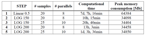
The following analysis have been compared:

• Two logarithmic with 150 frequencies analysed, with different number of parallels and samples;
• Two logarithmic with 200 frequencies analysed, with different number of parallels and samples.

In the following table are listed the analysis with their respective parameters, computational times and peak memory consumption.

Focusing on the g-acceleration along z-axis of a specific node, as can be seen from Figure 1, the trend for logarithmic coarser analysis is quite the same of the detailed one with linear step; this can also be verified by means of RMS value of the PSD (Power Spectral Density), the percentage differences from the detailed one is almost never beyond 10% and in the most of cases around 5%. For the specific node of this case study we have the following percentage differences:

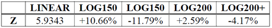
Figure 1

According to Figure 2 we can see that, for all the analysis, the problem is the loss of peak values, this is important, in particular for mid-lower frequencies up to 400Hz; this phenomenon is more evident for analysis 4 and 5 (LOG200), but depends on frequencies analysed – if are immediately after or before of a spike – and in particular to this node: increasing the number of frequencies the result will be more accurate.

Figure 2

In view of the results a good compromise between all analysis shown is the one with a logarithmic step for 150 frequencies, this allows to save 7 days compared to the most precise with step 0.5Hz, where frequencies analysed are 3981, but adding just 3.5 hours compared to a coarser one (LOG100); this allows the designer to have, since the beginning of the analysis, an idea of loads that the structure will be subjected of.

For this reason, taking into account of computational times and results accuracy, if the analyst wants to have an initial estimate of values that will occur in the structure, the suggestion is to use a lower value of samples and parallels with a sufficient number of frequencies analysed.

Modal and Direct Comparison

Since the beginning of this section emphasis must be placed on the high complexity of the direct analysis, this is due to the fact that the creation of the exterior acoustic mesh comes with an high RAM consumption and very long computational times; for this reason this kind of analysis cannot be done on a normal pc if we want to evaluate a wide band of frequencies (10 ÷ 2000Hz), even with 128Gb the analysis can stop if parameters are not set up well.

These problems are mainly connected to the creation of the finite and infinite fluid at lower frequencies: starting the analysis at 10Hz – according to the standard mesh criterion – means that the software has to create a bubble of 34m radius to be fitted with elements dependent on the upper frequency of its sub-band domain, differences from the upper and the lower sub domain can be seen in Figure 4 and Figure 5.

Figure 3

Figure 4

In Figure 6 are plotted results obtained for both the modal analysis of paragraph 2.1 with linear step of 0.5Hz and logarithmic for 150 frequencies and the direct analysis with logarithmic step for 80 frequencies.

It is noted that values are lower for the direct analysis, this may be due to the masking effect of the air surrounding the structure; the value of RMS of PSD in this case is less different from the modal detailed analysis then the coarser one is.

This analysis, although with few frequencies analysed took 6 days, quite the same computational time needed for the high detailed modal, and a peak memory consumption of 117Gb.

Figure 6

In conclusion, the advice is to use the modal analysis this allows to be conservative, furthermore, in order to save time and memory consumption launch the analysis with at least 150 frequencies with a logarithmic step to be analysed.

DIRECT FIELD ACOUSTIC NOISE TESTING SIMULATION

For the Acoustic Testing scenario, the excitation sources are noise generators like loudspeakers and horn-speaker, today’s standard practice is to use dedicated buildings like reverberant rooms, here the acoustic field is uniform and diffuse, the aim is to replicate the spectrum that the spacecraft will be subjected to during launch inside of the shroud. However there are many problems connected to this kind of test, in fact, the need to move the structure from various facilities, leads to increased costs and risks; for these reasons has been developed the DFAN (Direct Field Acoustic Noise), here the speakers and audio equipment can be easily trucked to different sites so it can be very portable, allowing convenience in spacecraft scheduling [3].

In order to achieve the acoustic levels and the diffuse field effects of a reverberation chamber, is important to have an acoustic field as uniform as possible, meaning the same SPL anywhere in the acoustic volume, the target of this simulation was to understand if the acoustic field around the structure was comparable to a properly diffuse field. In this analysis a 8x8x5m room filled with air elements has been created, than has been created 396 speakers all around the structure, in order to recreate a homogeneous field, results are shown in Figure 7.

Figure 7

Can be observed that the field is quite uniform in exception of two areas: the top of the satellite, probably due to a constructive interference, and the bottom, we can see a ground effect caused by the proximity of the satellite to the floor (0.5m) and is actually observed in the satellite testing phase.

The suggest for this test is to lift as possible the structure from the ground and not to put speakers over the maximum height of the satellite.

MSc Aerospace Engineering

Author: Mattia Cordaro

Supervisors: Prof. E. Carrera, Ing. D. Catelani, Prof. M. Cinefra, Prof. M. Petrolo